https://www.howtogeek.com/microsoft-excel-filter-unique-sortby-best-function-combination
Stop wasting hours manually sorting, deduplicating, and filtering your data in Excel. Instead, combine FILTER, UNIQUE, and SORTBY to create a self-cleaning data engine that does all the work from a single cell and never needs updating.
This function combination relies on dynamic arrays, which are only available in Excel for Microsoft 365, Excel 2021 or later, and Excel for the web.
How the FILTER-UNIQUE-SORTBY trio works
To create a list in Excel that is filtered, deduplicated, and alphabetized all at once, you need to stack these three functions together:
=SORTBY(
UNIQUE(FILTER(array,include,[if_empty])),
UNIQUE(FILTER(array,include,[if_empty])),
[sort_order]
)
Nested formulas can quickly become a wall of text. To create the line break shown above, press Alt+Enter in the formula bar. This doesn’t change how the formula works, but it makes it much easier to type and audit.
At first glance, you might notice that part of the formula repeats itself. This isn’t a mistake. To make this engine work without errors, you have to mirror the logic. I’ll explain exactly why we need to do this in Step 4 below.![]()
Related
The Beginner’s Guide to Nested Functions in Excel
Use multiple functions at the same time.
Step 1. The core: FILTER
Everything starts with FILTER, the engine room that identifies the raw data you want to extract:
FILTER(array,include,[if_empty])
- array is the range of cells or the table you want to filter.
- include is the criterion that tells Excel what to keep in the filter.
- [if_empty] (optional) is where you specify what Excel should display if no matches are found.
Instead of looking at a massive, messy table, FILTER identifies only the rows that meet your criteria. It ignores the noise and passes only the relevant data to the next step. What’s more, unlike the standard filter button, this doesn’t hide rows in your main table—it extracts them to a new location.
Step 2. The middle layer: UNIQUE
Next, UNIQUE acts as the “bouncer,” stripping away every duplicate from the filtered array it just received:
UNIQUE(FILTER(...))
In this trio, the entire result of the FILTER function serves as the only argument UNIQUE needs. By the time this layer is done, you have a clean list where every item appears exactly once. This is better than using the Remove Duplicates tool because it doesn’t affect your original table and doesn’t require a manual refresh if your source changes.
Step 3. The outer shell: SORTBY
The final step is the packaging. While UNIQUE is great for stripping out duplicates, it keeps the data in its original order. That’s where SORTBY comes in handy:
=SORTBY(array,sort_array,[sort_order])
- array is the result of the previous two steps.
- sort_array is the logic Excel uses to sort the list (see Step 4 below).
- [sort_order] (optional) tells Excel the direction of the sort. Use 1 for ascending (A-Z) or -1 for descending (Z-A). On the other hand, leave it blank to trigger the default (ascending).
While SORT works well for basic lists, SORTBY is the heavy-duty choice for two reasons. First, when stacking functions like UNIQUE and FILTER, SORTBY is better at handling spilled results without losing track of the data’s structure. Second, SORT only lets you sort by columns in your final result, whereas SORTBY allows you to sort your list based on a completely different column that isn’t even in your result.![]()
Related
SORT vs. SORTBY in Microsoft Excel: Which Should You Use?
Choose the best way to extract and rearrange your data in Excel.
Step 4. The mirror logic
Excel has a strict rule: the data you’re sorting and the criteria you’re sorting by must be exactly the same height. If your filtered unique list is five rows high, your sorting instructions must also be five rows high. So, if you tried to sort those five names using your original source table, the heights wouldn’t match, and the formula would break.
That’s why you need to mirror the logic by repeating the UNIQUE(FILTER(…)) chain as the second argument—you ensure the dimensions match perfectly every time.
=SORTBY(
UNIQUE(FILTER(array,include,[if_empty])), <-- the data to sort
UNIQUE(FILTER(array,include,[if_empty])), <-- the instructions to sort by
[sort_order]
)
The magic trio in action: The client list
Now that I’ve shown you the blueprint, let’s see the engine in action. Imagine you have an Excel table named T_Sales and want a live, alphabetized list of unique clients for the region selected in cell G2.
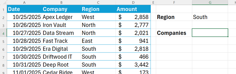
When you type this formula into cell G4, the formula spills its results down to the cells below:
Subscribe to the newsletter for Excel dynamic-array wins
Unlock practical Excel tools by subscribing to the newsletter: copyable dynamic-array formulas, mirrored SORTBY techniques, and spill-range fixes you can paste into workbooks. Also discover related function combos to build reliable data engines.
Subscribe
By subscribing, you agree to receive newsletter and marketing emails, and accept our Terms of Use and Privacy Policy. You can unsubscribe anytime.
=SORTBY(
UNIQUE(FILTER(T_Sales[Company],T_Sales[Region]=G2,"No Matches")),
UNIQUE(FILTER(T_Sales[Company],T_Sales[Region]=G2,"No Matches")),
1
)
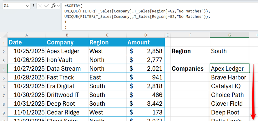
Referencing a cell rather than hard-coding the filter into the formula means that you can easily switch to a different region. It also makes your engine easier for others to understand: they don’t need to know how SORTBY works—they just need to know to type or choose a region from a drop-down list in cell G2.
Because the original dataset is in an Excel table, the data engine is future-proofed. If you add new rows of sales data to the bottom of the table, the formula automatically detects the expanded range. This is one of the benefits of using functions that spill dynamic arrays from the cell where you typed the formula. What’s more, you can reference the entire result elsewhere just by adding a hash (#)—also known as a spilled range operator—to the reference:
G4#

Related
Everything You Need to Know About Structured References in Excel
Use table and column names instead of cell references.
Final pitfalls to avoid
To keep your new data engine running smoothly, keep these three rules in mind:
- Clear the path: Dynamic array formulas need empty space to spill their results downward. If a stray piece of text or another table is in the way, Excel will throw a #SPILL! error.
- No formulas inside tables: While you should use a table as your source data, your formula must sit in a regular cell. This is because Excel tables don’t support dynamic spilling.
- Leave a one-column buffer: When analyzing data outside an Excel table, always leave a one-column gap between the table and where you’re typing. Otherwise, Excel thinks you’re adding more data to your table, so it will “grab” your analysis.
By moving away from manual Excel tools and embracing dynamic arrays, you build systems that grow alongside your data. This trio is the perfect starting point for exploring other Excel function combinations—such as INDEX with XMATCH, IF with AND and OR, and EOMONTH with SEQUENCE—that can further automate your daily tasks.