https://www.howtogeek.com/microsoft-excel-sumifs-function
Microsoft Excel’s SUMIFS function calculates the sum of values in a range of cells based on multiple conditions. It avoids the need for complex filtering, and its conditions can be numbers, text, or dates, making it great for dynamic data analysis.
The SUMIFS function is available to those using Excel 2016 or later, Excel for Microsoft 365, Excel for the web, or the Excel mobile and tablet apps.
The Difference Between SUMIF and SUMIFS
The best way to see how SUMIF and SUMIFS differ is to compare their syntaxes.
Here’s the SUMIF syntax:
=SUMIF(a,b,[c])
where
- a (required) is the range to be tested,
- b (required) is the criterion for the above range, and
- c (optional) is the range containing the values to sum.
You only need to include argument c if the range containing the values to sum differs from the range containing the values to be tested. If you omit argument c, Excel will sum the values in the range identified in argument a.
Now, let’s see how that differs from the SUMIFS syntax:
=SUMIFS(a,b¹,b²,[c¹,c²,...])
where
- a (required) is the range of cells to sum,
- b¹ and b² (required) form the first range-criterion pairing, where b¹ is the range to be tested, and b² is the criterion, and
- c¹ and c² (optional) form the first of up to 126 additional range-criterion pairings.
If you find that you only need to use arguments a, b¹, and b², you might consider using the SUMIF function instead. However, the benefit of sticking with SUMIFS is that the formula is ready for further criteria you could add down the line.
So, there are three key differences between SUMIF and SUMIFS:
- SUMIF lets you specify only one condition, while SUMIFS lets you specify many.
- The argument containing the range to sum is optional at the end of the SUMIF syntax, while the same argument is mandatory at the start of the SUMIFS syntax.
- The ranges tested for each criterion must be the same size as the range of cells to sum when using the SUMIFS function, whereas there’s no such requirement with the SUMIF function.
Using SUMIFS With Numbers
The SUMIFS function in Excel is great for summing the values in a column based on multiple numerical criteria.
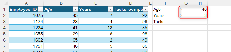
In this Excel table, named T_Staff, column A contains employee ID numbers, column B contains employees’ ages, column C contains the number of years each employee has worked for the company, and column D details the number of tasks each employee has completed.
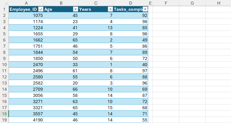
Let’s imagine you want to aggregate the tasks completed based on age (column B) and number of years of service (column C). Specifically, you want to work out the total number of tasks completed by employees over 40 with more than three years of experience.
To do this, in a blank cell, type:
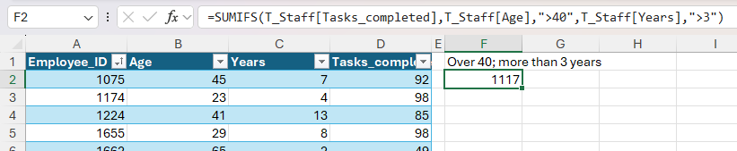
=SUMIFS(T_Staff[Tasks_completed],T_Staff[Age],">40",T_Staff[Years],">3")
where
- T_Staff[Tasks_completed] tells Excel that you want to sum the values in the Tasks_completed column of the T_Staff table,
- T_Staff[Age],”>40″ tells Excel to search the Age column for values greater than 40, and
- T_Staff[Years],”>3″ tells Excel to search the Years column for values greater than 3.
Logical expressions with comparison operators (like >, <, >=, <=, and <>) should always be enclosed in double quotes (“”). Otherwise, if the criteria are exact numerical matches, you can simply type the number.
Only on rows where the two criteria are met will the values in the Tasks_completed column be summed.
Here’s what you get when you press Enter:
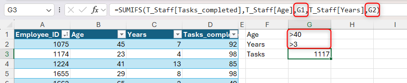
That’s great, but at the moment, the conditions are hard-coded, meaning if you want to change them, you have to edit the formula. That’s why you should place the criteria in separate cells, and reference those cells in the formula instead:
=SUMIFS(T_Staff[Tasks_completed],T_Staff[Age],G1,T_Staff[Years],G2)
This formula produces the same result as the hard-coded formula, but now, you can easily change the parameters in cells G1 and G2. What’s more, placing the logical operators in the referenced cells avoids the need to use double quotes.
Let’s go one step further and make the formula even more dynamic by separating the logical operators from the numerical conditions.
Now, you can use the ampersand (&) symbol in the formula to concatenate the logical operators and the numerical conditions:
=SUMIFS(T_Staff[Tasks_completed],T_Staff[Age],G1&H1,T_Staff[Years],G2&H2)
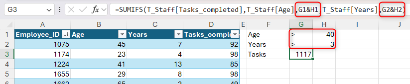
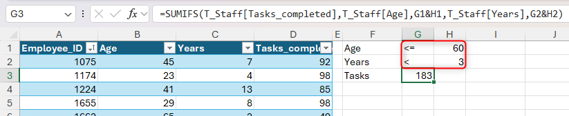
As a result, not only can you quickly change the numerical parameters in cells J9 and J10, but you can also switch logical operators in cells I9 and I10. In this example, the formula returns the number of tasks completed by employees aged 60 or less with fewer than three years’ experience:
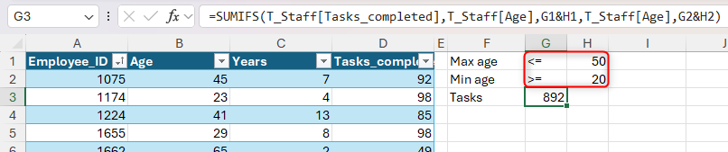
Finally, you can use SUMIFS to sum values whose corresponding cells fall within a range. For example, typing:
=SUMIFS(T_Staff[Tasks_completed],T_Staff[Age],G1&H1,T_Staff[Age],G2&H2)
sums the values in the Tasks_completed column for staff aged between 20 and 50, inclusive.
Using SUMIFS With Text (And Wildcards)
The SUMIFS function works in a similar way with text as with numbers, but there are two key differences. First, text in Excel formulas must always go inside double quotes, and second, you can use wildcards for partial matches.
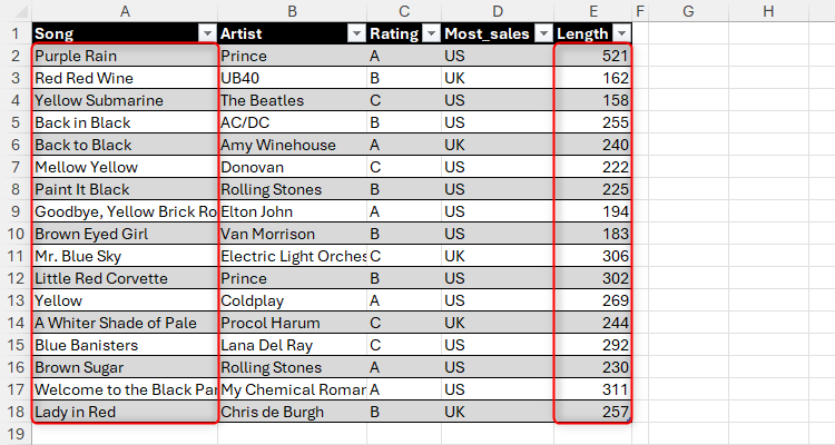
Suppose you’re creating a playlist from a list of songs in the Excel table named T_Songs.
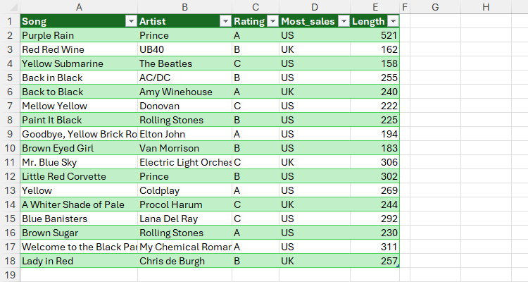
Specifically, you want to work out the duration of a playlist that includes A-rated songs that sold the most copies in the U.S.
To do this, type:
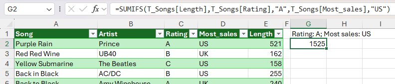
=SUMIFS(T_Songs[Length],T_Songs[Rating],"A",T_Songs[Most_sales],"US")
where
- T_Songs[Length] tells Excel to sum the values in the Length column of the T_Songs table,
- T_Songs[Rating],”A” tells Excel to search the Rating column for the text value A, and
- T_Songs[Most_sales],”US” tells Excel to search the Most_sales column or the text value US.
Notice how all the text values in the formula are wrapped in double quotes. Otherwise, Excel will assume it’s searching for numerical values, so it will return an error.
Here’s the result when you press Enter:
Remember, however, that formulas are more dynamic when referencing cells containing the conditions. This formula returns the same result:
=SUMIFS(T_Songs[Length],T_Songs[Rating],H1,T_Songs[Most_sales],H2)
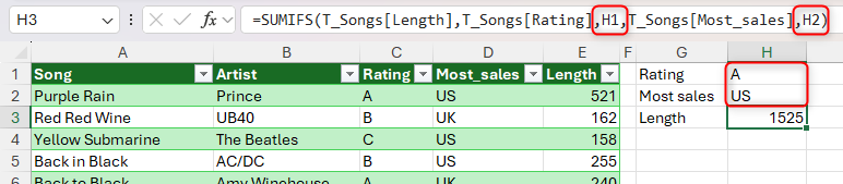
As you can see in the formula above, another benefit of referencing cells instead of hard-coding the criteria is that, most of the time, you can omit the double quotes, making the formula quicker to produce and easier to read.
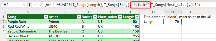
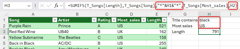
In a second example, let’s imagine you want to work out the length of a playlist of songs containing the text string black that sold the most copies in the U.S. This is where wildcards come into play:
=SUMIFS(T_Songs[Length],T_Songs[Song],"*black*",T_Songs[Most_sales],"US")
Here, “*black*” tells Excel that the criterion for the Song column of the T_Songs table is any text value (hence the double quotes) containing black. Each asterisk (*) represents any number of characters—in other words, the text string black can have any number of characters before or after, meaning it can appear in any part of a song’s title.
On the other hand, there’s no need for wildcard characters for the second criterion (US) because we’re looking to return a whole match, not a partial one.
Here’s the reference-style alternative:
=SUMIFS(T_Songs[Length],T_Songs[Song],"*"&H1&"*",T_Songs[Most_sales],H2)
This time, the asterisk wildcard characters are each placed inside double quotes and concatenated with the cell reference using ampersand (&) signs, ultimately representing the string *black* as in the previous formula.
The other wildcard character in Excel is the question mark (?), which represents any single character. Also, if you want to include asterisks or question marks in criteria as characters in their own right, place a tilde (~) before them.
Using SUMIFS With Dates
An overlooked use of the SUMIFS function is summing a range based on date criteria.
This Excel table, named T_Tasks, contains various projects, their cost, and their completion due dates.
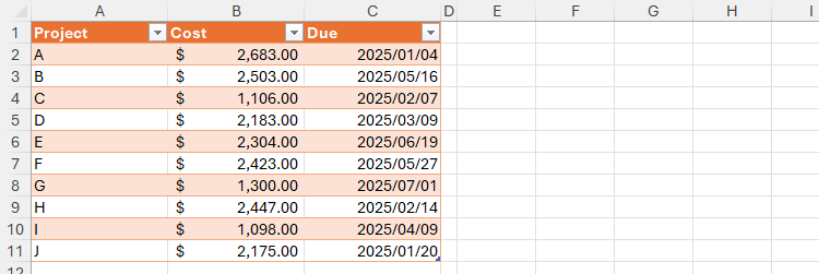
Your aim is to work out the cost of all projects due in February and March 2025.
As I’ve explained in all the examples above, referencing cells rather than hard-coding conditions is often the better method, not only because it makes the formula dynamic, but also because the formulas are cleaner. This is especially the case with dates, where Excel is very particular about the format in which they’re entered.
So, here’s the reference-based formula you should insert for this scenario:
=SUMIFS(T_Tasks[Cost],T_Tasks[Due],F1&G1,T_Tasks[Due],F2&G2)
where
- T_Tasks[Cost] is the column containing the values to sum,
- T_Tasks[Due],F1&G1 concatenates the greater-than-or-equal-to logical operator in cell F1 (which represents later than or on the same day as) and the start date in cell G1 to define the earliest date to look up in the Due column, and
- T_Tasks[Due],F2&G2 concatenates the less-than-or-equal-to logical operator in cell F2 (which represents earlier than or on the same day as) and the end date in cell G2 to define the latest date to look up in the Due column.
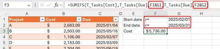
In the above screenshot, a custom date number format is applied to cells G1 and G2, and the accounting number format is applied to cell F3.
Using SUMIFS With OR Logic
By default, the SUMIFS function works with AND logic—in other words, the values in the range identified by argument a are only summed when all the criteria in the subsequent arguments are met.
However, with a few tweaks to the formula, you can introduce OR logic, where the values in the specified range are summed when one of multiple criteria is met.
Let’s go back to the T_Songs table, but this time, you want to calculate the total length of all songs whose titles contain the text strings red or black.
One way to achieve this is to use array constants, which you must enclose in curly braces:
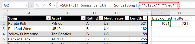
=SUMIFS(T_Songs[Length],T_Songs[Song],{"*black*","*red*"})
where
- T_Songs[Length] is the column containing the values to sum,
- T_Songs[Song] is the range containing the values you want to evaluate, and
- {“*black*”,”*red*”} searches that column for the text strings black or red.
When you press Enter, you get a spilled dynamic array of two results, because Excel effectively evaluates the Song column twice—once for the text string black, and once for the text string red—returning each result in separate cells.
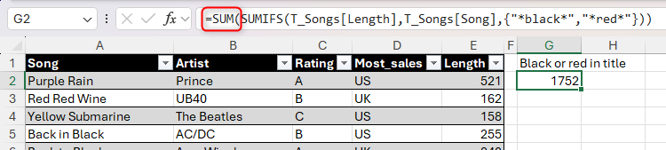
However, since the aim is to yield a single result, you need to nest the whole formula inside the SUM function:
=SUM(SUMIFS(T_Songs[Length],T_Songs[Song],{"*black*","*red*"}))
The drawback of this method is that you can’t use cell references inside array constants, meaning you have to hard-code the criteria.
To get around this, you could combine multiple SUMIFS formulas using the add (+) sign. I’ve split the formula below onto separate lines so that you can clearly see how each part works:
=SUMIFS(T_Songs[Length],T_Songs[Song],"*"&H1&"*")
+
SUMIFS(T_Songs[Length],T_Songs[Song],"*"&J1&"*")
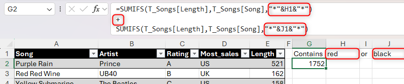
However, this structure results in a lengthy formula if you have several OR criteria, so bear this in mind before deciding which method to use.
Excel consulting ; Excel Consulting – Consultoria em Excel e Office 365